Numerical simulation: ODE/PDE solver and spin-up
For Earth Science model development, I inevitably have to deal with ODE and PDE equations. I also have come across some discussion related to this Researchgate Question.
In an attempt to answer this question, as well as redefine the problem I am dealing with, I decided to organize some materials to illustrate our current state on this topic.
Models are essentially equations. In Earth Science, these equations are usually ODE or PDE. So I want to discuss this from a mathematical perspective.
Ideally, we want to solve these ODE/PDE with initial condition (IC) and boundary condition (BC) using various numerical methods:
Because of the nature of geology, everything is similar to its neighbors. So we can construct a system of equations which may have multiple equation for each single grid cell. Now we have an array of equations with the same number of knowns and unknowns. We can solve them simultaneously using numerical methods. In this case, we are not using “spin-up” at all. In fact, lots of models do not use spin-up to reach steady state, e.g., three-dimensional groundwater model MODFLOW.
For example, let’s imagine a single cube and corresponding model in space as below:
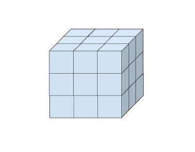
\begin{equation} \frac{ \partial Q }{ \partial t } = f(Q) + f(w) + … + Source - Sink \end{equation}
where $Q$ is unknown system state variable, i.e., storage; $f(Q)$ is storage related process; $f(w)$ is other processes; $Source$ is source; and $Sink$ is sink.
In most cases, the $f(Q)$ depends on local gradient, which means that:
\begin{equation} f(Q) = f(Q_{i,j}, Q_{i-1,j}, …) \end{equation}
With certain boundary condition (BC), we can write an array of equations:
\begin{equation} \label{equ:matrix}
\begin{bmatrix}
\frac{ \partial Q_{0,0} }{ \partial t } \\
\frac{ \partial Q_{1,0} }{ \partial t } \\
\frac{ \partial Q_{2,0} }{ \partial t } \\
\frac{ \partial Q_{i,j} }{ \partial t }
\end{bmatrix} =
\begin{bmatrix}
f(Q_{0,0}) + f(w_{0,0}) + … + Source_{0,0} - Sink_{0,0} \\
f(Q_{1,0}) + f(w_{1,0}) + … + Source_{1,0} - Sink_{1,0} \\
f(Q_{2,0}) + f(w_{2,0}) + … + Source_{2,0} - Sink_{2,0} \\
f(Q_{i,j}) + f(w_{i,j}) + … + Source_{i,j} - Sink_{i,j}
\end{bmatrix}
\end{equation}
In some simple scenarios, we can solve the equations above directly. For example, when $Q_{i,j}$ is the only unknown, the total unknowns and number of equations are the same. In this case, we might be able to solve the equations using a direct solver (MUMPS, etc.).
However, as our models grow more complicated, e.g., CESM. Our ODE and PDE are getting more complex when all the terms on the right hand side are more complicated. Existing direct solver methods may not suit for the equation solving any more. So instead of solving the equation directly, we can solve the equation using iterations (PETSc, etc.).
However, even for iterative solver, it can take a long computing time to find a “solution”. So we have another “solution”, we can let the system to evolve through time naturally. And this process is often called “spin-up”. In this scenario, we can use spin-up to approximate $Q_{i,j}$ with initial condition (IC).
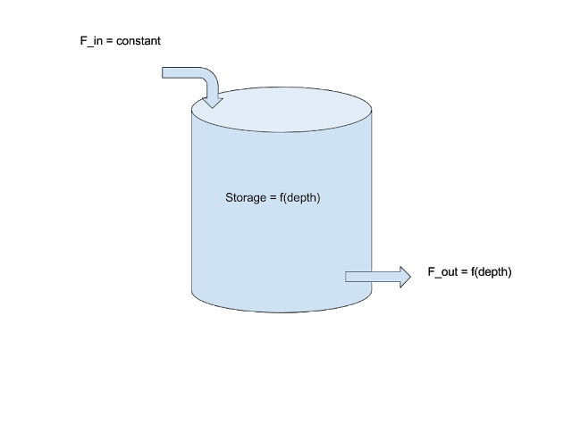
Regardless of the initial condition, the system will gradually converge to “steady state”. For example, regardless how much water is stored in the tank initially, the water will reach the same level after certain time when inflow equals outflow.
 You can easily setup much complicated scenarios similar to:
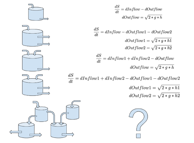
When you have multiple pools and flux terms, the system may become very sensitive to certain parameters.
Illustration of ODE with 8 buckets. Each bucket is contributing water into other buckets at different rates. Each bucket has different storage capacity and radius.
Besides, if you take a close look at most numerical methods, they usually use iteration/time step to reach solution. Therefore, they are actually very similar to spin-up but with different time steps.
The criteria which is used to determine whether the system is in “steady state” is also critical. More often we expect a state variable does not change significantly with time, then we say this system is in “steady state”. However, any threshold has a limit, needless to say that seldom a system is in absolute steady state.
Because of the complexity of the system, a spin-up can be trapped inside a local valley/hilltop similar to:
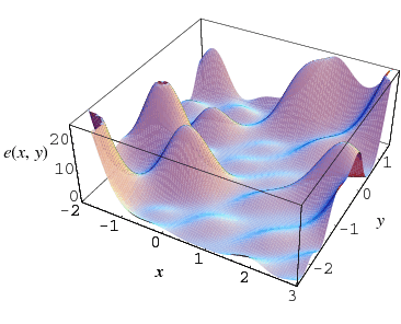
In this case, our “criteria” must be carefully defined, but that is out of the scope of this discussion.
Getting back the equation, even though we may list as many as equations in the matrix, there are no more than 27 equations associated with each cube in a 3D space because there are only 26 neighbors for each cube. As a result, after we estimated the system state variable using spin-up, we no longer need to solve a matrix of equations anymore and we can directly calculate all terms just like spin-up process.
So here comes the question: when do we still need numerical methods to solve ODE/PDE equations?
I believe a side by side comparison will make it easier to understand the fundamental idea behind different approaches.
Let’s start with the classical heat equation:
https://en.wikipedia.org/wiki/Heat_equation
There is also a very nice program online to demonstrate the equation: http://people.sc.fsu.edu/~jburkardt/cpp_src/fd1d_heat_explicit/fd1d_heat_explicit.html If you compare the formula with above discussion, then we should realize that this method is very similar to “spin-up”.
But as the title implies, this is an explicit method, specifically, an explicit finite difference method, which is widely used in numerical simulation.
https://en.wikipedia.org/wiki/Finite_difference_method
“In mathematics, finite-difference methods (FDM) are numerical methods for solving differential equations by approximating them with difference equations, in which finite differences approximate the derivatives. FDMs are thus discretization methods. Today, FDMs are the dominant approach to numerical solutions of partial differential equations”
However, how we approximate the derivatives determines the accuracy of the method and explicit apparently has least accuracy compared with implicit and other methods.
In general, “the implicit scheme is always numerically stable and convergent but usually more numerically intensive than the explicit method as it requires solving a system of numerical equations on each time step.”, that is why we seldom use implicit methods on large modeling system such as CESM.
To summarize, “spin-up” is an explicit Euler forward finite difference method and most linear/nonlinear matrix solvers are implicit finite difference methods. You can find the advantage and disadvantage of both methods easily.