A visual decomposition of the land grid in the E3SM/CESM model
One of my recent development projects needs to exchange several variables between different components using the Common Infrastructure for Modeling the Earth (CIME) model. However, different components have different grid systems. Therefore, I have to get familiar with the grid system of these two component before assigning any variables.
One of them is the land grid used in Community Land Model (CLM)/ELM, which is the land component in the Energy Exascale Earth System Model (E3SM) model. Because CLM is also part of CESM, this post should also apply to the CESM land component.
In short, the land component distributes all the land units across multiple nodes/cores and each grid cell is run by clump.
Here I developed a small Python utility to illustrate the concept.
First we define a sample problem as follow:
| Variable | Value | Description |
|---|---|---|
| npes | 4 | CPU/Node |
| clump_pproc | 10 | Core per CPU |
| nsegspc | 2 | Segment per clump |
| nclumps | 40 | Core count |
| lni | 20 | Longitude count |
| lnj | 10 | Latitude count |
| numg | 85 | Land count |
Then we define the global grid and land mask:
Before you start to read the numbers, you need to understand the index system used in E3SM. Even though Fortran is a column-major language, the E3SM (written in Fortran) stores the global grid using a row-major approach. As a result, global grid index starts from left to right in memory, same as the land mask (Figure 1).
Note that yellow square represent clump index, blue square represent land index, and red square represents global grid index.
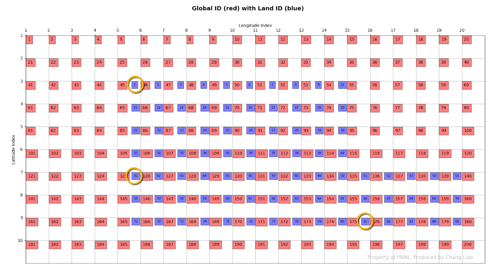
Figure 1. The global ID and land ID map.
Similar to global grid, clump/core index starts from left to right across node/processor. For example, clump 1 is located on the first core on processor 1 and clump 2 is located on the first core on processor 2.
Last, we distribute the land grid onto the clumps. All the land grids are allocated to clump in order. In the end, a clump may simulate multiple land grids which are far away in the spatial domain. For example, the clump 1 simulates land grid 1, 41 and 81 (circled in yellow in Figure 1 and 2).
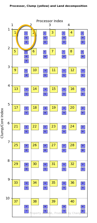
Figure 2. The processor, clump and land grid decomposition.
The global grid and land grid is connected through the “gdc2glo” variable, which stores what is the land grid index for each clump in order. For example, gdc2glo[1] = 125 means that the 125th global grid is the “second” (index starting from 0) simulated land grid, which is land grid 41.
Let me know if you have any question.